Script de simulation Scilab
fr -
eng
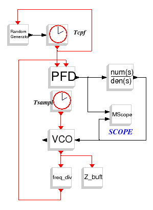
Jigue de phase de sortie d'un synthťtiseur de frťquence ŗ rapport de division entier N
synthe_int_jit_sim.cos
scs_m.props.context=[
'F_cpf = 20e6;'
'T_cpf = 1/F_cpf;'
'sig_ref=T_cpf*0.1/100'
'Fo = 2.045e9;'
'To = 1 / Fo;'
'wo=2*%pi * Fo;'
'kv = 100.5e6;'
'alpha=6.91e9;'
'beta2=0.15;'
'Fd=2.44e9;'
'N=int(Fd/F_cpf)'
'j_vco=10e6;'
'Nsampl = 2;'
'Tsampl = To/Nsampl;'
'Fsampl = 1 / Tsampl;'
'Icp = 5e-3;'
'Ileak=0;'
'Ileak_sig=1e-6;'
'fn=F_cpf/180;'
'phi=%pi/4;'
'[tau1,tau,tau2]=calcul_3eme_ordre(fn,phi,kv*2*%pi,Icp,N);'
's=poly(0,''s'');'
'num=1+tau1*s;'
'den=tau*s*(1+tau2*s);'
'Nsav=10000'
'Tfin=Nsav*Tsampl*30'
];
synthe_int_jit_sim_ctxt.sce
//Define simulation name
sim_name='synthe_int_jit_sim';
//Define simulation path
sim_path='synthe_int_jit_sim';
//Load scicos diagram
load(MODNUMCOS+'/examples/simu/'+sim_path+'/'+sim_name+'.cos');
//Define context
exec(MODNUMCOS+'/examples/simu/'+sim_path+'/'+sim_name+'_ctxt.sce');
context=scs_m.props("context");execstr(context);
//Define Simulation end time
scs_m.props.tf=Tfin;
//Define other variables
j=1;
//substitue context variable to be sweep
//scs_m.props.context=subst_ctxt('varname','varname=');
//Initialise Info and %scicos_context variable
clear Info;Info=list();
clear %scicos_context;
%scicos_context=struct();
//Do simulation with scicos_simulate
Info=scicos_simulate(scs_m,Info,%scicos_context);
//Load result
myvar=return_state_block(Info,"z_buft");
f=scf(10);
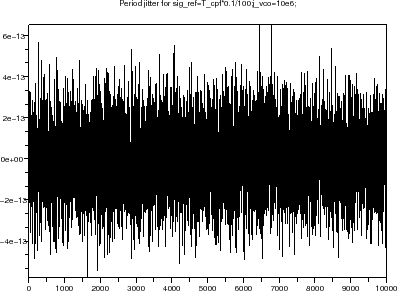
plot2d(1:Nsav,myvar(1)(1:Nsav)-1/Fd,rect=[0 min(myvar(1)(1:Nsav)-1/Fd) Nsav max(myvar(1)(1:Nsav)-1/Fd)]);
xtitle('Period jitter for '+scs_m.props.context(3)+';'+scs_m.props.context(12));
g=scf(20);
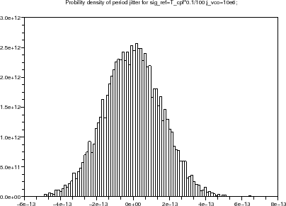
histplot(100,myvar(1)(1:Nsav)-1/Fd);
xtitle('Probility density of period jitter for '+scs_m.props.context(3)+';'+scs_m.props.context(12));
synthe_int_jit_sim.sce
Figure : (a) Courant de sortie de la pompe de charge; Tension d'entrťe du VCO
Figure : (b) Evolution du jitter pťriodique
Figure : (c) Densitť de probabilitť du jitter pťriodique
A. Layec