Scicos Diagram
fr - eng


Duffing's oscillator

\epsfig{file=duffing_diagr.eps,height=12cm}

Module


Contents

Description

The Duffing's equation is described by this nonlinear differential equation :

\begin{eqnarray}
\frac{y\left(t\right)}{dt}&=&x\left(t\right)-x^{3}\left(t\right)-\epsilon y\left(t\right)+\gamma\cos\left(\omega t\right)
\end{eqnarray}


where $ \epsilon$ and $ \gamma$ are parameters and $ \omega$ a pulsation.
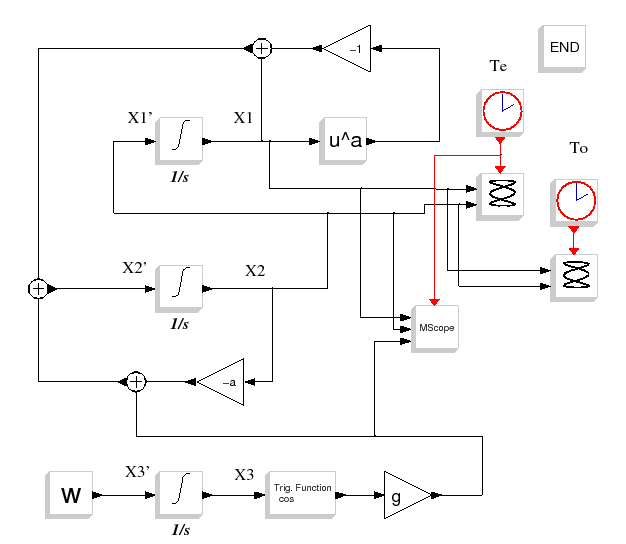
This forced oscillator should be written as a three dimensional state equation system :

\begin{eqnarray}
\tilde{x_{1}}&=&x_{2}\\
\tilde{x_{2}}&=&x_{1}-x_{1}^{3}-\epsilon y+\gamma\cos\left(x_{3}\right)\\
\tilde{x_{3}}&=&\frac{2\pi}{T}
\end{eqnarray}


Context


Te   = 0.02
g    = 0.3
a    = 0.15
w    = 1
To   = 2*%pi/w
ci1  = 0.1
ci2  = 0.1
ci3  = 0
Tfin = 400
 

Scope Results

\begin{figure}\begin{center}
\epsfig{file=duffing_scope_1.eps,width=330.00pt}
\end{center}\end{figure}
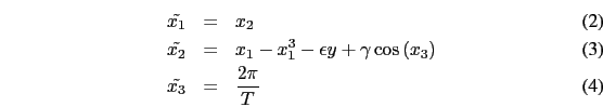
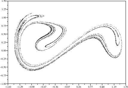
Figure : (a) Phase plan

\begin{figure}\begin{center}
\epsfig{file=duffing_scope_2.eps,width=330.00pt}
\end{center}\end{figure}
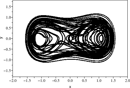
Figure : (b) Time domain waveforms

\begin{figure}\begin{center}
\epsfig{file=duffing_scope_3.eps,width=330.00pt}
\end{center}\end{figure}
Figure : (c) Poincare section

Authors

A. Layec