chua_diagr

Scicos Diagram
fr - eng

Chua's system

$\epsfig{file=chua_diagr.eps,width=400pt}$

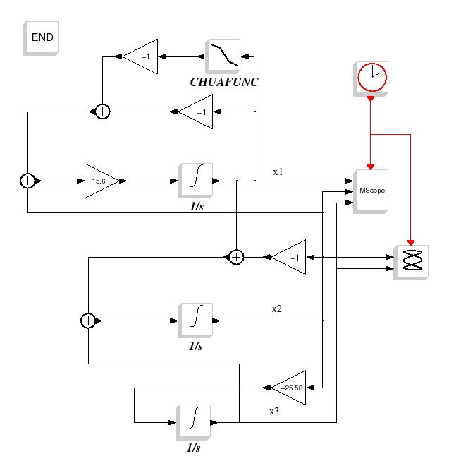
This diagram does the simulation of the Chua's chaotic system.
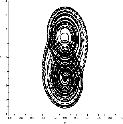
Over the past few years, this system have been many studed to detail synchronization principles of chaotic systems. He is originally realized with the electronic circuit shown in the following figure.

$\begin{figure}\centering \scalebox{0.8}{% \input{chua_circuit.pstex_t}} \end{figure}$

Figure 1: Chua's circuit

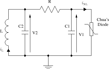
This circuit is composed with passive elements (L,C1,C2,R) and with an active nonlinear element (a diode).
It is described by the following system of equations of continuous state variables :

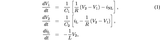
$\begin{eqnarray} \frac{dV_{1}}{dt}&=&\frac{1}{C_{1}}\left[\frac{1}{R}\left(V_{2}... ...\nonumber\\ \frac{di_{\rm L}}{dt}&=&-\frac{1}{L}V_{2}, \nonumber \end{eqnarray}$

$\begin{eqnarray} f(V_{1})&=&G_{\rm b}\, V_{1}+\frac{1}{2}\left[G_{\rm a}-G_{\rm ... ...eft\vert V_{1}+E\right\vert-\left\vert V_{1}-E\right\vert\right]. \end{eqnarray}$

By changing parameters with $\alpha=\dfrac{C_{2}}{C_{1}}$ , $\beta=\dfrac{C_{2}}{L}R^{2}$ , $m_{0}=\dfrac{G_{\rm a}}{R}$ , $m_{1}=\dfrac{G_{\rm b}}{R}$ and renaming state variables, the new system of nonlinear equations is :

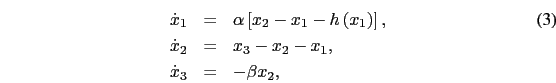
$\begin{eqnarray} \dot{x}_{1}&=&\alpha\left[x_{2}-x_{1}-h\left(x_{1}\right)\right... ...}-x_{2}-x_{1}, \nonumber\\ \dot{x}_{3}&=&-\beta x_{2}, \nonumber \end{eqnarray}$

and the nonlinearity :

$\begin{eqnarray} h(x)&=&m_{1}\, x+\frac{1}{2}\left[m_{0}-m_{1}\right]\, \left[\left\vert x+E\right\vert-\left\vert x-E\right\vert\right], \end{eqnarray}$

that's the system realized by the Scicos diagram for :

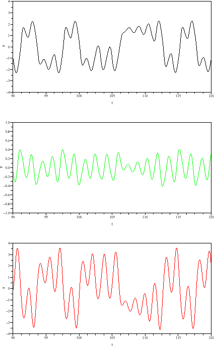
$\begin{eqnarray} \left[\alpha;\beta;m_{0};m_{1};E\right]&=&\left[15.6;25.58;8/7... ...\left[1.6;0;-1.6\right] \;\;\rm {(initial\;conditions).}\nonumber \end{eqnarray}$

Context

//**coef of chua's function**//
m0 = -8/7
m1 = -5/7

//**init. conditions of state variables**//
ci = [1.6;0;-1.6]

//**sampling period**//
Tsampl = 1e-2

//**final time simulation**//
Tfin = 120